Canonical & Correspondence Analysis
Block Matrices

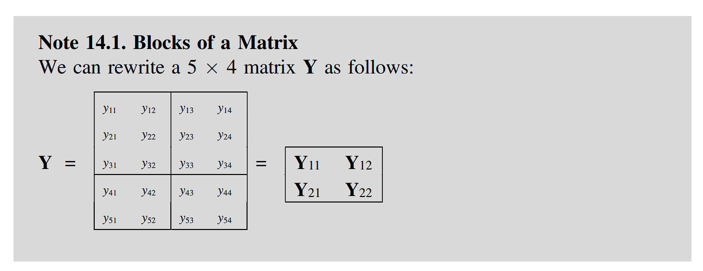
where: \(\mathbb{Y_{11}, Y_{12}, Y_{21}, Y_{22}}\) are called blocks of Y, while Y is called a block matrix consisting of \(\mathbb{Y_{11}, Y_{12}, Y_{21}, Y_{22}}\).
Here, a block matrix of data is arranged horizontally:
\[\mathbb{X}=\begin{bmatrix} \mathbb{X_1, \cdots, X_j, \cdots, X_J} \end{bmatrix}\]and a block matrix of parameters is arranged vertically:
\[\mathbb{C}=\begin{bmatrix} \mathbb{C_1} \\ \vdots \\ \mathbb{C_j} \\ \vdots \\ \mathbb{C_J} \end{bmatrix}\]where \(\mathbb{X_j, C_j}\) are called the jth block of X and C, respectively.
\[\mathbb{XC}=\sum_{j=1}^{J}\mathbb{X_jC_j}=\mathbb{X_1C_1}+ \cdots + \mathbb{X_JC_J}\]Canonical Correlation Analysis
Let’s consider an n-individuals-p-variables data matrix \(\mathbb{X=[X_1, X_2]}\) consisting of two blocks \(\mathbb{X_1}=[\vec{x_{11}}, \cdots, \vec{x_{1p_1}}](n \times p_1)\) and \(\mathbb{X_2}=[\vec{x_{21}}, \cdots, \vec{x_{2p_2}}](n \times p_1)\). That is, the p variables in X are classified into a group of \(p_1, p_2\) variables.
Canonical correlation analysis (CCA) with two blocks is formulated as minimizing
\[\tag{1} \begin{equation} f(\mathbb{C_1, C_2})=\lVert \mathbb{X_1C_1-X_2C_2} \rVert^2 \end{equation}\]subject to
\[\frac{1}{n}\mathbb{C_1^TX_1^TX_1C_1}=\frac{1}{n}\mathbb{C_2^TX_2^TX_2C_2}=\mathbb{I_m}\]That is, the purpose of CCA is to obtain the coefficient matrices C1 and C2 that allow X1C1 and X2C2 to be mutually best matched.
When \(m=1\), the correlation coefficient between X1c1 and X2c2 is expressed as
\[\frac{n^{-1}\vec{c_1}\mathbb{X^T_1X_2}\vec{c_2}}{\sqrt{n^{-1}\vec{c_1}\mathbb{X^T_1X_1}\vec{c_1}}\sqrt{n^{-1}\vec{c_2}\mathbb{X^T_2X_2}\vec{c_2}}}\]This particular coefficient is called a canonical correlation coefficient between the variables in X1 and those in X2.
Multivariate Categorical Data
An example of multivariate categorical data is given by a 5-individuals by 3-variables matrix \(Y = (y_{ij})\), where the variables are
- Faculty to which each individual belongs
- Subject at which she/he is best
- Sciences, basic or applied, to which she/he is oriented
Here, after dummifying the original categorical multivariables, it expands into a wider matrix, which is labelled as G, called membership matrix.
Multiple Correspondence Analysis
The loss function for multiple correspondence analysis (MCA) is given by
\[\tag{2} \eta(\mathbb{F, C})=\sum_{j=1}^{J}\lVert \mathbb{F-G_jC_j} \rVert^2\]subject to constrain
\[\mathbb{F=JF}\]Discriminant Analysis
Doscriminant analysis refers to a group of statistical procedures for analyzing a daya set with individuals classified into certain groups, where the resutls of the analysis are used for finding the group of a new individual that is not included in the previous data set.
Modification of Multiple Correspondence Analysis: Canonical Discriminant Analysis
The multiple correspondence analysis (MCA) i sperformed for the n-individuals by K-categories membership matrix G. Let J=1, and G=G1, and an n-individuals by p-variables quantitative data matrix X corresponding to G** is given. The data set is expressed as an \(n \times (K+p)\) block matrix \(\mathbb{[G, X]}\).
For example, individuals are irises whose categories are indicated by G and the individuals’ features are described by X:
\[\begin{bmatrix} 1 & 0 & 0 & −0.90 & 1.02 & −1.34 & −1.31 \\ 0 & 1 & 0 & −1.14 & −0.13 & −1.34 & −1.3 \\ \vdots & \vdots & \vdots & \vdots & \vdots & \vdots & \vdots \\ 1 & 0 & 0 & 0.07 & −0.13 & 0.76 & 0.79 \end{bmatrix}\]Modified based MCA
\[\tag{3} \mathbb{F=GC} \Rightarrow \eta(\mathbb{B,C})=\lVert \mathbb{XB-GC} \rVert^2\]subject to constrain of
\[\frac{1}{n}\mathbb{B^TX^TXB}=\mathbb{I_m}\]Minimizing (3) over B, C subject to the constrain is called canonical discriminant analysis.
Comparison to Cluster Analysis
Deleting B from the loss function (3) leading to the objective function of cluster analysis.
- the matrix G, which indicates the memberships of individuals to groups, is known in discriminant analysis
- G is unknown and to be obtained in cluster analysis
- Therefore, discriminant analysis is called supervised classification, while cluster analysis is called unsupervised classification.
Enjoy Reading This Article?
Here are some more articles you might like to read next: